17 SciPy + Statsmodel

1 Introduction

SciPy and Statsmodels are complementary Python libraries widely used for statistical analysis, but they serve different purposes within the analytical workflow.

• SciPy (scipy.stats) provides core statistical functionality, including probability distributions, summary statistics, and classical hypothesis tests such as t-tests, chi-square tests, and ANOVA. It is typically used for standalone inferential procedures.
• Statsmodels is designed for statistical modeling and inference. It offers a unified framework for estimating regression models, conducting hypothesis tests within models, and performing diagnostic checks, with a formula interface similar to R.
• Practical distinction: Use SciPy when the goal is to perform individual hypothesis tests. Use Statsmodels when the objective is to model relationships among variables and obtain detailed inferential output.

Load data:

import numpy as np
import pandas as pd
penguins = pd.read_csv("data/penguins.csv").dropna()
penguins.head()

	species	island	bill_length_mm	bill_depth_mm	flipper_length_mm	body_mass_g	sex	year
0	Adelie	Torgersen	39.1	18.7	181.0	3750.0	male	2007
1	Adelie	Torgersen	39.5	17.4	186.0	3800.0	female	2007
2	Adelie	Torgersen	40.3	18.0	195.0	3250.0	female	2007
4	Adelie	Torgersen	36.7	19.3	193.0	3450.0	female	2007
5	Adelie	Torgersen	39.3	20.6	190.0	3650.0	male	2007

2 One Sample \(t\) Test

Importing scipy.stats:

from scipy import stats

Research question: Is the mean body mass different from 4000 g?

stats.ttest_1samp(penguins["body_mass_g"], popmean=4000)

TtestResult(statistic=np.float64(4.6924522789847325), pvalue=np.float64(3.952443195315995e-06), df=np.int64(332))

Decision rule: Reject \(H_0\) if \(p < 0.05\).

---

3 Independent Two Sample \(t\) Test

Research question: Do male and female penguins differ in mean body mass?

male = penguins.loc[penguins.sex == "male", "body_mass_g"]
female = penguins.loc[penguins.sex == "female", "body_mass_g"]

stats.ttest_ind(male, female, equal_var=False)

TtestResult(statistic=np.float64(8.554537231165762), pvalue=np.float64(4.793891255051492e-16), df=np.float64(323.89588102864843))

---

4 Chi Square Test of Independence

Research question: Is species associated with sex?

table = pd.crosstab(penguins["species"], penguins["sex"])
stats.chi2_contingency(table)

Chi2ContingencyResult(statistic=np.float64(0.04860717014078318), pvalue=np.float64(0.9759893689765846), dof=2, expected_freq=array([[72.34234234, 73.65765766],
       [33.69369369, 34.30630631],
       [58.96396396, 60.03603604]]))

---

5 One Way ANOVA

Research question: Does mean body mass differ across species?

adelie = penguins.loc[penguins.species == "Adelie", "body_mass_g"]
chinstrap = penguins.loc[penguins.species == "Chinstrap", "body_mass_g"]
gentoo = penguins.loc[penguins.species == "Gentoo", "body_mass_g"]

stats.f_oneway(adelie, chinstrap, gentoo)

F_onewayResult(statistic=np.float64(341.8948949481461), pvalue=np.float64(3.74450512630046e-81))

---

6 Simple Linear Regression

Statsmodels uses a formula interface similar to R, which simplifies handling of categorical variables and interactions.

Model: Body mass predicted by flipper length

import statsmodels.formula.api as smf

model1 = smf.ols(
  "body_mass_g ~ flipper_length_mm",
  data=penguins
).fit()

model1.summary()

OLS Regression Results

Dep. Variable:	body_mass_g	R-squared:	0.762
Model:	OLS	Adj. R-squared:	0.761
Method:	Least Squares	F-statistic:	1060.
Date:	Sat, 21 Feb 2026	Prob (F-statistic):	3.13e-105
Time:	00:24:52	Log-Likelihood:	-2461.1
No. Observations:	333	AIC:	4926.
Df Residuals:	331	BIC:	4934.
Df Model:	1
Covariance Type:	nonrobust

	coef	std err	t	P>|t|	[0.025	0.975]
Intercept	-5872.0927	310.285	-18.925	0.000	-6482.472	-5261.713
flipper_length_mm	50.1533	1.540	32.562	0.000	47.123	53.183

Omnibus:	5.922	Durbin-Watson:	2.116
Prob(Omnibus):	0.052	Jarque-Bera (JB):	5.876
Skew:	0.325	Prob(JB):	0.0530
Kurtosis:	3.025	Cond. No.	2.90e+03

Notes:
[1] Standard Errors assume that the covariance matrix of the errors is correctly specified.
[2] The condition number is large, 2.9e+03. This might indicate that there are
strong multicollinearity or other numerical problems.

---

7 Multiple Linear Regression

model2 = smf.ols(
  "body_mass_g ~ flipper_length_mm + bill_length_mm + C(sex)",
  data=penguins
).fit()

model2.summary()

OLS Regression Results

Dep. Variable:	body_mass_g	R-squared:	0.807
Model:	OLS	Adj. R-squared:	0.805
Method:	Least Squares	F-statistic:	457.1
Date:	Sat, 21 Feb 2026	Prob (F-statistic):	5.89e-117
Time:	00:24:52	Log-Likelihood:	-2426.7
No. Observations:	333	AIC:	4861.
Df Residuals:	329	BIC:	4877.
Df Model:	3
Covariance Type:	nonrobust

	coef	std err	t	P>|t|	[0.025	0.975]
Intercept	-5433.5336	286.558	-18.961	0.000	-5997.251	-4869.816
C(sex)[T.male]	358.6309	41.572	8.627	0.000	276.851	440.411
flipper_length_mm	48.2093	1.841	26.179	0.000	44.587	51.832
bill_length_mm	-5.2012	4.860	-1.070	0.285	-14.762	4.360

Omnibus:	0.549	Durbin-Watson:	1.751
Prob(Omnibus):	0.760	Jarque-Bera (JB):	0.664
Skew:	0.081	Prob(JB):	0.718
Kurtosis:	2.852	Cond. No.	3.03e+03

Notes:
[1] Standard Errors assume that the covariance matrix of the errors is correctly specified.
[2] The condition number is large, 3.03e+03. This might indicate that there are
strong multicollinearity or other numerical problems.

---

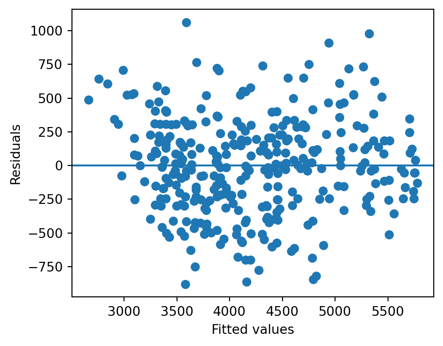
8 Residual Diagnostics

import matplotlib.pyplot as plt

resid = model2.resid
fitted = model2.fittedvalues

plt.scatter(fitted, resid)
plt.axhline(0)
plt.xlabel("Fitted values")
plt.ylabel("Residuals")
plt.show()

---

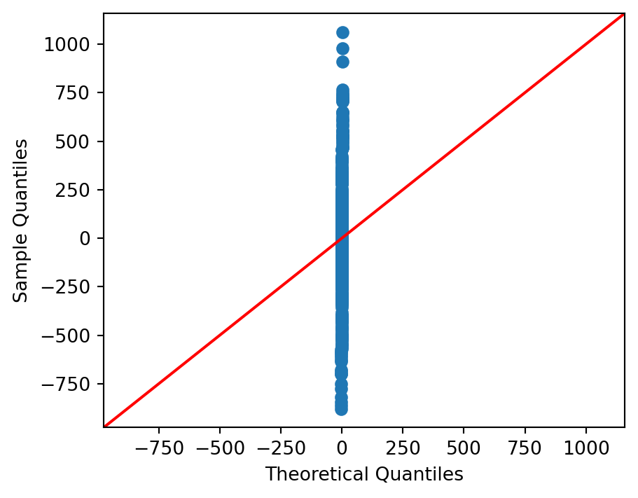
9 Normality of Residuals

import statsmodels.api as sm

sm.qqplot(resid, line="45")
plt.show()