print("Hello, Python!")Hello, Python!(CSE331) Python for Data Science
Python is a general-purpose programming language widely used in:
Python was created by Guido van Rossum and first released in 1991. It was initially developed at the Centrum Wiskunde & Informatica (CWI) in the Netherlands.
Python is popular because it has:
The development of Python is supported by the Python Software Foundation (PSF) and a large community of contributors.
A traditional first program is:
print("Hello, Python!")Hello, Python!Python can also be used as a calculator:
2 + 3510 * 550(12 + 8) / 45.0Python treats uppercase and lowercase letters as different characters.
For example, name, Name, and NAME are three different names.
Python provides tools for almost every stage of a data-science project:
Some packages that we will use in this course are:
| Package | Main purpose |
|---|---|
| NumPy | Numerical arrays and mathematical operations |
| pandas | Data manipulation using data frames |
| Matplotlib | Basic data visualization |
| Seaborn | Statistical data visualization |
| Plotly | Interactive visualization |
| SciPy | Scientific and numerical computing |
| statsmodels | Statistical models and hypothesis tests |
| scikit-learn | Machine-learning models and utilities |
In some programming workflows, analysts use one language for data exploration and another language for building the final application.
Python can often be used for both:
When additional speed is required, Python packages can use optimized implementations written in languages such as C, C++, or Fortran.
This is sometimes discussed as the two-language problem: one language is used for analysis and another for production. Python can reduce the need to switch between languages.
Python can be downloaded directly from:
https://www.python.org/downloads/
However, installing Python alone does not automatically install every package or interface needed for data science.
For this course, we will use Anaconda Distribution because it provides:
conda package manager; andDownload Anaconda Distribution from:
https://www.anaconda.com/download
Choose a current version of Python 3. Python 2 is obsolete and should not be used for this course.
Open Anaconda Prompt, Terminal, or Command Prompt and enter:
python --versionDepending on the operating system, one of the following commands may be required:
python3 --versionpy -3 --versionYou can also check whether JupyterLab is installed:
jupyter lab --versionPython provides an interactive environment in which commands can be entered and executed immediately.
From a terminal, run:
pythonOn some systems, use:
python3You should see a prompt similar to:
>>>This interactive environment is called the Python interpreter, Python shell, or Python REPL.
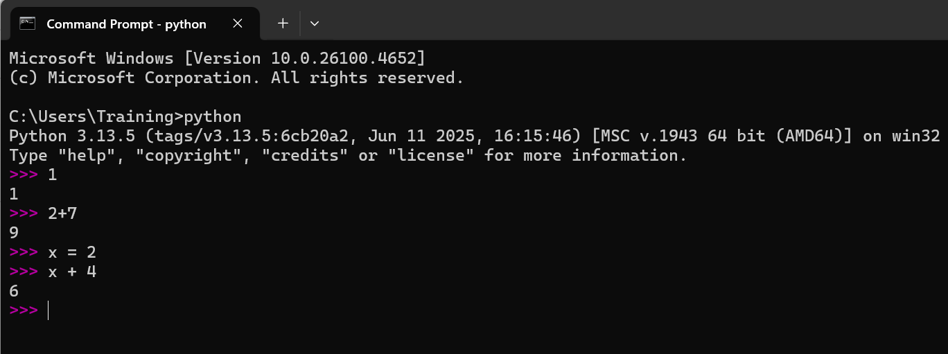
REPL stands for Read–Evaluate–Print Loop.
For example:
>>> 5 + 7
12
To exit the REPL, enter:
exit()You may also press Ctrl+D on macOS/Linux or Ctrl+Z, followed by Enter, on Windows.
Python code can be written and executed in several ways.
A Python script is a plain-text file containing Python code. Its filename usually ends with .py.
For example:
analysis.pyA script can contain:
name = "Rasel"
print("Hello,", name)
Popular editors and integrated development environments for Python scripts include:
A console provides an interactive prompt in which commands are executed one at a time.
It is useful for:
A Jupyter notebook is an interactive document that can contain:
A notebook file normally ends with:
.ipynbFor example:
lecture_01.ipynbJupyterLab is the browser-based interface that we will use to create and manage notebooks.
The distinction is important:
Open Anaconda Prompt or a terminal and enter:
jupyter labJupyterLab should open automatically in your default web browser.
The terminal window must normally remain open while JupyterLab is running.
To stop JupyterLab:
Ctrl+C; andWe will primarily use JupyterLab in this course. The classic command
jupyter notebookopens a different notebook interface.
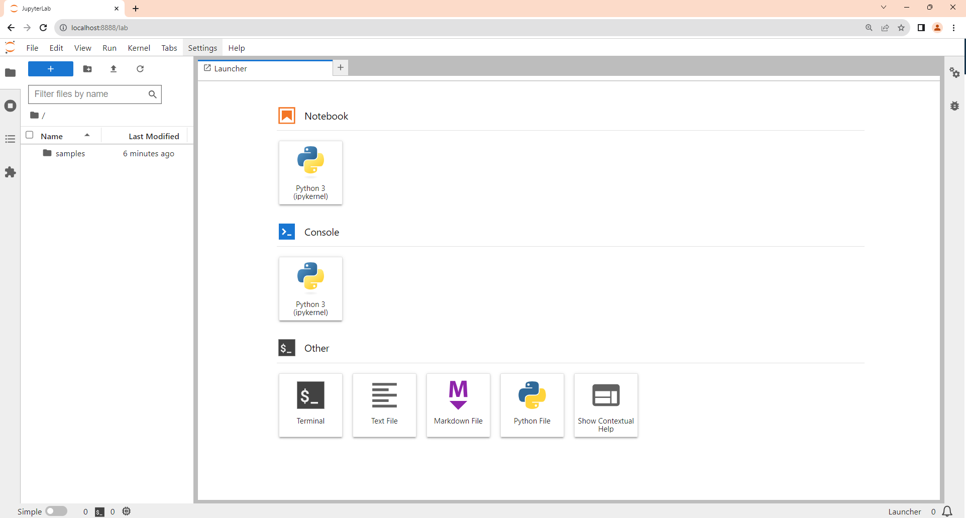
The JupyterLab interface usually contains:
From the launcher, you can open a:
To create a new notebook:
JupyterLab initially gives the notebook a name such as:
Untitled.ipynb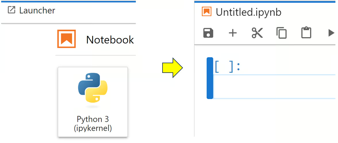
Rename it to something meaningful, such as:
lecture_01_practice.ipynbTo rename a notebook:
A notebook uses a kernel to execute code.
The kernel:
For this course, we will normally use a Python kernel.
The kernel remains active until it is:
A Jupyter notebook is divided into rectangular sections called cells.
The two most important cell types are:
A code cell contains Python code.
For example:
x = 10
y = 5
x + y15The result appears directly below the cell.
A code cell may contain:
A Markdown cell contains formatted text rather than Python code.
Markdown cells can be used for:
For example:
# Main Heading

## Subheading

This is **bold text** and this is *italic text*.

- First item
- Second itemThe most common keyboard shortcut is:
Shift+Enter: run the current cell and move to the next cell.Other useful shortcuts are:
| Shortcut | Action |
|---|---|
Shift+Enter |
Run the cell and move to the next cell |
Ctrl+Enter |
Run the cell and remain in the same cell |
Alt+Enter |
Run the cell and insert a new cell below |
Enter |
Enter edit mode |
Esc |
Enter command mode |
In command mode, the following shortcuts are useful:
| Shortcut | Action |
|---|---|
A |
Insert a cell above |
B |
Insert a cell below |
M |
Change the cell to Markdown |
Y |
Change the cell to code |
D, D |
Delete the selected cell |
Z |
Undo cell deletion |
Some browser or operating-system shortcuts may interfere with JupyterLab shortcuts. Commands are also available from the JupyterLab menus.
Create a code cell and enter:
student_name = "Ayesha"
course = "Python for Data Science"

print("Student:", student_name)
print("Course:", course)
Student: Ayesha
Course: Python for Data ScienceNow perform a calculation:
quiz_1 = 8
quiz_2 = 9
assignment = 10

total = quiz_1 + quiz_2 + assignment
total27A notebook displays the result of the final expression automatically.
Compare:
total27with:
print(total)27Both display the value, but print() explicitly asks Python to display it.
Jupyter Markdown cells support mathematical notation written using LaTeX syntax.
Inline mathematics is placed between single dollar signs:
The sample mean is denoted by $\bar{x}$.It appears as:
The sample mean is denoted by \(\bar{x}\).
Display mathematics is placed between double dollar signs:
$$
\bar{x} = \frac{1}{n}\sum_{i=1}^{n}x_i
$$
It appears as:
\[ \bar{x} = \frac{1}{n}\sum_{i=1}^{n}x_i \]
Notebook cells do not necessarily run from top to bottom automatically.
Suppose the following cell is run first:
result = value * 2Python will produce an error if value has not already been defined.
The required cell must be run first:
value = 10After that, the calculation will work:
result = value * 2
result
The number beside a code cell, such as [1], [2], or [3], indicates its execution order.
A well-organized notebook should work when its cells are run from the first cell to the last cell in order.
Before submitting a notebook, use:
Kernel → Restart Kernel and Run All Cells
Then check whether every cell runs without an error.
A cell may sometimes take too long to finish.
To stop the current calculation, use:
Kernel → Interrupt Kernel
If the notebook behaves unexpectedly, use:
Kernel → Restart Kernel
Restarting the kernel:
After restarting, the cells must be run again.
JupyterLab usually saves notebooks automatically, but it is good practice to save your work manually.
Use:
Ctrl+S on Windows/Linux; orCommand+S on macOS.Good notebook filenames include:
lecture_01_practice.ipynb
assignment_01.ipynb
household_data_analysis.ipynb
Avoid filenames such as:
new final latest notebook 2.ipynbPrefer:
The working directory is the folder Python currently treats as its main location for reading and writing files.
For example, when Python reads:
data.csvit normally searches for that file in the current working directory.
Use the os module:
import os

os.getcwd()
The result may look like:
C:\Users\Student\Documents\python_courseor:
/Users/student/Documents/python_courseTo list files and folders in the current directory:
import os

os.listdir()On Windows:
import os

os.chdir(r"C:\Users\Student\Documents\python_course")
On macOS or Linux:
import os

os.chdir("/Users/student/Documents/python_course")
The r before a Windows path creates a raw string, which helps Python interpret backslashes correctly.
A better habit is to create a separate folder for each project and launch JupyterLab from that folder. This reduces the need to change the working directory repeatedly.
IPython and Jupyter provide special commands called magic commands.
These commands usually begin with %.
%pwdThe %pwd command displays the working directory.
%lsThe %ls command lists files in the current directory.
%cd /path/to/folderThe %cd command changes the working directory.
Magic commands are features of IPython and Jupyter. They are not part of standard Python and may not work inside an ordinary .py script.
A module is a file containing reusable Python code.
A package is a collection of related modules.
Packages allow us to use functions and tools developed by other programmers without writing everything ourselves.
Community-contributed Python packages are commonly distributed through the Python Package Index, or PyPI.
A package must usually be imported before it can be used.
import mathWe can then use functions from that package:
math.sqrt(25)5.0Data-science packages are often imported using standard abbreviations:
import numpy as np
import pandas as pd
import matplotlib.pyplot as plt
import seaborn as sns
Here:
np represents NumPy;pd represents pandas;plt represents matplotlib.pyplot; andsns represents Seaborn.These abbreviations are conventions rather than requirements.
A package must be installed only once in a particular Python environment. However, it must be imported again whenever a new Python session begins.
Inside Jupyter, use:
%pip install package_nameFor example:
%pip install emojiThe %pip command is generally preferable to writing only pip inside a notebook because it installs the package into the Python environment associated with the active kernel.
Using pip:
python -m pip install package_nameOn some systems:
python3 -m pip install package_nameUsing conda from Anaconda Prompt:
conda install package_nameAfter installing a package, you may sometimes need to restart the notebook kernel.
Install the emoji package:
%pip install emojiImport and use it:
import emoji

message = emoji.emojize(
    "Python is :thumbs_up:",
    language="alias"
)

print(message)
Expected result:
Python is 👍Errors are a normal part of programming. An error message provides information about what went wrong.
For example:
print(student_age)--------------------------------------------------------------------------- NameError Traceback (most recent call last) Cell In[12], line 1 ----> 1 print(student_age) NameError: name 'student_age' is not defined
Because student_age has not been defined, Python returns a NameError.
Read an error message from the bottom upward. The final line normally gives:
Common errors during the first few lectures include:
| Error | Possible reason |
|---|---|
NameError |
A variable has not been defined |
SyntaxError |
The code does not follow Python syntax |
ModuleNotFoundError |
A required package is not installed |
FileNotFoundError |
Python cannot find the requested file |
TypeError |
An operation was applied to an unsuitable data type |
Do not be afraid of error messages. Learning to understand and correct errors is an essential programming skill.
When working with notebooks:
In this lecture, we learned that:
%pip can be used to install packages from a notebook.Before the next class, make sure that you can: